Continuous functions - general concepts

The discrete probability distributions addressed earlier involved an assigned probability for each possible value in a distribution.

In contrast, continuous probability distribution functions have continuous values between a lower limit and an upper limit and so it is not possible to assign a probability to a specific score or value. Instead we determine the probability for a range of observations.

Continuous probability distributions.

For a continuous probability distribution, the two main characteristics are:

no probability value can be negative;
the total area defined by a distribution must be 1.0. So something will happen.

Common basic questions used for continuous function contexts are:

1. Determine if a function is a PDF.
This is always answered by showing the total area under the function between the limits is 1.0

2. Use the PDF to find probabilities within defined domains.
This question is always answered by using integration between the given limits.

3. Expected value and variance questions.
These questions are answered by integrating:
* the product of x times the pdf (for expected value); and
* x² times the pdf to obtain E(x²) then the usual Var (x) = E(x²) - [E(x)]² (for the variance).
Both of these approaches are very similar to the approaches used for discrete probabilty functions.

Uniform probability distributions.

A uniform probability distribution function - f(x) or P(x) - is constant for all possible values of x. That is the graph is a straight line between the minimum and maximum values of the variable being used and at a constant height showing the probability of that event occurring.

The following diagram is a typical example of a uniform distribution: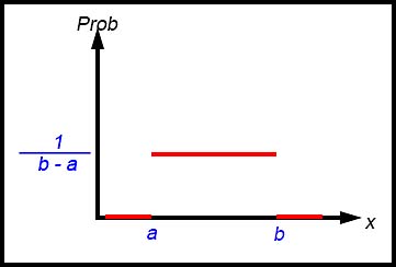

The uniform distribution defines equal probabilities over a given reference range for the continuous distribution - in this case between x = a and
x = b. The probabilities are then calculated as 1 divided by the difference between the upper and lower values - so 1/(b - a). If a = 4 and b = 9,
(b - a) = 5 so each probability throughout the range is 0.2.

To find probabilities for uniform distributions, we calculate the areas of rectangles.

Pr (4 < x < 6) = difference between the two given values divided by 5 = 2/5 = 0.4.

The expected value for a uniform distribution is calculated in the same way as for the usual continuous distributions using integrations of the product of x and the probabilty:

As there is no term in x, this approach is used for all continuous uniform probability distributions.

The variance is calculated in the same way as is usual - that is using x² not x in the term to be integrated.
See Probability Density functions TYS 1 Q 14. The value is .

Other continuous probability distribution functions.

More common continuous probability distributions vary in their probabilities across the range of values for the variable. These distributions can take any form although lines, parabolas and exponentials are common basic shapes.

The probability that the value of a random variable X lies between h and k is the area under the function between h and k. To find that area for a continuous function requires integrating the function between the limits h and k.

NOTE: It is not possible to use a continuous PDF to calculate the probability of a specific number occuring because the area of a line drawn at that point is zero. So P(X = 2) = 0. Be careful of this sutuation because it can be a TRICK QUESTION in a mutiple choice context.

Also notice there is no difference in the answer to P(1<X≤2) or the answer to P(1≤X≤2). Another trick question.